Six ways to score generated order flow
The same continuations. Different comparisons. This guide follows the Wasserstein scoring path from input trajectories to feature scores and aggregates. Shared operations are black; a different colour marks what each protocol changes.
Two meanings of “conditional”
| When? | What is conditioned on? | Example | What changes? |
|---|---|---|---|
| During generation | Historical context supplied to the model | Read 250 real events, then generate 250 new events | History influences the generated continuation, including through the model's inference state |
| During scoring | Features measured from the completed real and generated continuations | Group observations by spread, then compare best-ask volume within each group | The observations entering each distribution comparison |
These are separate choices. Feature-conditioned scoring does not ask the model to regenerate data at a specified spread or volatility. Here, a continuation means events after the historical context, not a later phase of training.
| Description when generation uses historical context | Scoring mode on this page | Comparison |
|---|---|---|
| Context-conditioned, marginal | feature_marginal | Compare the overall feature distributions, pooling across histories |
| Context-conditioned, feature-conditioned | feature_conditional | Compare target-feature distributions within groups defined by a conditioning feature |
Both descriptions assume historical context was supplied during generation. Neither scoring mode preserves the identity of each history–future pair; that is the purpose of context_paired.
Naming and implementation status. The two-word names below are explanatory names. Existing CLI identifiers remain listed alongside them; the unified rename is not yet deployed. context_paired is a new local implementation, defaulting to one generated continuation per history. It is not a new set of measured leaderboard results and does not retroactively change historical scores.
| Name | Existing identifier | Description |
|---|---|---|
| feature_marginal | uncond | Pool observations across histories |
| context_paired | Separate new launcher | Keep each history paired with its future |
| feature_conditional | cond | Group by continuation features |
| context_binned | context | Derive boundaries from historical context |
| time_lagged | time_lagged | Offset the conditioning and target features |
| temporal_divergence | divergence | Slice generation into successive windows |
Six methods at a glance
Choose a method by the question it answers. All six can score continuations generated from historical context; what differs is how observations are compared after generation. The table describes the implementations documented here, including the new local paired scorer.
| Method | What does it ask? | What is compared? | How are scores combined? | Main advantage | Main limitation |
|---|---|---|---|---|---|
| feature_marginal | Do generated features look realistic overall? | Pool real feature observations across histories; separately pool generated observations. Compare the two distributions for each feature. | One normalized Wasserstein distance per feature; equal mean of all 21 valid feature scores for WS21. | Broad, simple check of overall feature distributions; useful as a first diagnostic. | Pooling loses history identity and can hide incorrect relationships between features. More observations mean more weight; matching marginals does not imply realistic trajectories. |
| context_paired | Does a generated future resemble the observed future associated with the same history? | Keep each history’s real and generated continuation paired; compare their feature distributions separately. Default: one generated continuation per history. | Compute distances first, then average equally across histories. An optional cross-feature mean requires supplied fixed reference scales; default feature set has 4 features. | Preserves historical pairing and exposes mismatches that pooling can conceal. Each history has equal weight. | One observed future is only one possible outcome. With one generated sample, distance cannot establish conditional calibration and may penalize legitimate variability; feature summaries still omit aspects of event order. |
| feature_conditional | Are relationships such as spread given volatility realistic? | Group each side by its own continuation-condition values, using shared boundaries; compare target distributions inside each group. | Normalize within each group, then weight by real-plus-generated observation counts. Three configured feature-pair scores; no automatic WS21-style mean across pairs. | Detects relationships that can be wrong even when overall marginal distributions match. | Does not retain historical pairing. Results depend on binning and coverage; sparse or missing groups complicate interpretation. Tests only the configured relationships. |
| context_binned | Do continuation features match within regimes whose boundaries are calibrated from historical data? | Derive boundaries from historical contexts, then group real and generated observations by their own continuation features. | Within-group normalized distances, weighted by real-plus-generated counts. One default pair: best-ask volume given spread. | Anchors the boundary construction in historical observations instead of pooled future conditions. | It does not assign each future to its own history’s regime and is not a per-history comparison. Default coverage is narrow; bin sparsity and missing-group issues remain. |
| time_lagged | Are later features consistent with earlier feature conditions? | Append context to each continuation; align feature arrays; pair a later target with an earlier condition, then group. Default lag: 500 aligned positions. | Within-group normalized distances, weighted by real-plus-generated counts. Three configured lagged feature-pair scores. | Checks temporal relationships that same-stage feature comparisons can miss. | Sensitive to lag and feature alignment; short paths may be skipped and some targets may still lie in historical context. Pooling loses history identity; it is not a causal test. |
| temporal_divergence | Does generated feature realism change as generation progresses? | Split generated continuations into successive windows; compare each stage with the pooled, full real-continuation reference. Default window: 100 events. | A distance curve per feature. An optional declared mean at each stage requires all 21 features; stages are not automatically averaged. | Shows where generation drifts or deteriorates instead of hiding the pattern in a single overall score. | Real and generated windows are not matched by stage. Window length, feature availability and changing normalization can affect the curve, so a change is not necessarily model deterioration alone. |
For feature_conditional, context_binned and time_lagged, the current code skips undefined group scores without renormalizing their weights. Report the covered weight alongside the score. Scores across these six protocols are not directly interchangeable because their comparison units, weighting and normalization differ.
0. Shared inputs and notation
How to read every operator
| Symbol | Read it as | Exact operation |
|---|---|---|
| \(A\uplus B\) | concatenate, preserving duplicates | Join two lists. Repeated observations remain repeated. Order does not affect the empirical distribution. |
| \(\biguplus_{i=1}^{M} A_i\) | concatenate all indexed lists | Join \(A_1,A_2,\ldots,A_M\). Unlike a sum, the result is a list, not a number. |
| \(\delta_a\) | point mass at \(a\) | A probability distribution that places all its probability at the value \(a\). |
| \(\mathcal E(A)\) | empirical distribution of \(A\) | Give each observation in the list probability \(1/\lvert A\rvert\). Equal-valued observations add their probability masses. |
| \(\ldots\), \(\cdots\), \(\vdots\) | continue the same pattern | Omitted intermediate items, horizontally or vertically. |
| \(\Vert\) | append in temporal order | Join a history and a continuation as an ordered trajectory. Unlike \(\uplus\), its time order is essential. |
| \([a:b]\) | zero-based slice | Include positions \(a\) through \(b-1\); exclude the right endpoint \(b\). |
| \(\operatorname{Pool}\) | pool feature observations | Concatenate the underlying observations and construct their empirical distribution. Trajectories with more observations receive more mass. |
Subscripts identify an item; a superscript such as \(f\) identifies a feature, not a power. Parenthesized superscript \((k)\) identifies a generated member. A hat, as in \(\widehat P\), denotes an estimate from observed data. A superscript \(\star\) labels a fixed reference quantity; it does not indicate multiplication. Superscripts such as “paired” or “marginal” are protocol labels, not exponents.
One history, one observed future, possibly many generated futures
Let \(i=1,\ldots,M\) index historical contexts. \(C_i\) contains \(L\) observed events. \(R_i\) is its one realized continuation of \(T\) events. Each \(G_i^{(k)}\) is a separately sampled continuation from that same context, not a subdivision of a single continuation.
| Symbol | Meaning |
|---|---|
| \(M\); \(i\) | Total number of historical contexts; index of one context, from 1 to \(M\). |
| \(L\); \(T\) | Number of events in a history; number of events in a continuation. |
| \(C_i\); \(R_i\) | Historical event sequence; its observed future event sequence. |
| \(K_i\); \(k\) | Number of generated continuations for history \(i\); generated-member index. |
| \(G_i^{(k)}\) | The entire \(k\)-th generated continuation for history \(i\). |
| \(\theta\) | The model parameters, held fixed during generation and scoring. |
| \(p_\theta(\cdot\mid C_i)\) | The model's distribution over possible future sequences given history \(C_i\). |
For example, \(L=T=1000\) means 1,000 historical events followed by 1,000 future events. It is an illustration, not a requirement of every benchmark artifact. The new paired protocol requires a common continuation event count within a scoring run.
Reading \(K\) throughout this guide. \(K_i\) always counts complete generated continuations for history \(i\), not events, bins, feature pairs or generation windows. Write \(K_i=K\) only when every history has the same count. For the existing modes, the number must be read from the run's generation manifest or matched generated file pairs; it cannot be inferred from the mode name. This guide specifies supported counts, not an audited numerical count for every historical leaderboard artifact.
Independent repeated generation should restore the same context state before each sample and vary the sampling randomness. A start token alone does not establish whether historical information was used.
Default K: mode-by-mode and feature-by-feature source map
\(K_i\) counts generated continuations for history \(i\). The inspected base-model inference writes one continuation per history (\(K_i=1\)). The original five scoring modes have no separate numerical K default: they consume the generated members supplied by the loader. The new paired launcher enforces K = 1 unless ensemble scoring is explicitly requested. Feature counts, bin counts, context lengths and continuation lengths are separate quantities.
| Mode | Default feature coverage | K with this inference output | Scorer behavior | Source consuming members |
|---|---|---|---|---|
| feature_marginal | 21 features | 1 for every feature | All supplied members | scoring.py:88 → partitioning.py:263–275 |
| context_paired | 4 features | 1 | Enforces one member by default | run/benchmarking/run_context_paired.py:42–46 |
| feature_conditional | 3 feature pairs | 1 for every pair | All supplied members | scoring.py:134–145 → partitioning.py:263–275 |
| context_binned | 1 feature pair | 1 | All supplied members | scoring.py:478–485 → partitioning.py:263–275 |
| time_lagged | 3 feature pairs | 1 for every pair | Iterates over supplied members | scoring.py:225 (worker), scoring.py:347 (serial) |
| temporal_divergence | Same 21 features, by stage | 1 | Slices each member; stages do not increase K | scoring.py:573–575; partitioning.py:95 |
Shared source locations and how K is read
Short filenames in these tables are under src/lobpipeline/scorer/lob_bench/. Paths refer to the inspected sigma-0 source revisions in Section 8.
| Shared source | Exact operation | Interpretation |
|---|---|---|
| src/base_model/inference/generate.py:2188–2194 | Writes real_id_{i}_gen_id_0 message/book files | One continuation per history; 0 is the member index |
| data_loading.py:482–485 | Matches real_id_{real_id}_gen_id_*.csv | Collects available generated members |
| data_loading.py:558 | num_gen_series=(len(gmp),) | K is read from the input files, not configured per feature |
| partitioning.py:263–275 | Applies each feature function to seq.m_gen and seq.b_gen | Different features reuse the same generated continuations |
| run/benchmarking/run_context_paired.py:44 | expected_k = args.expected_k if args.ensemble else 1 | Paired scoring enforces K = 1 by default |
| src/lobpipeline/lob_bench/context_paired_io.py:70–95 | Rejects multiple members in single-sample mode unless a fixed ID is selected | No silent best-member selection |
K for each feature and configuration location
Each row below inherits K = 1 from the inspected inference output; the original feature configurations do not individually fix K. With other input files, the original modes use the loader's actual member count instead.
| Mode | Feature / target–condition pair | K with inspected inference | Configuration location |
|---|---|---|---|
| feature_marginal / temporal_divergence | spread | 1 | run_bench.py:28 |
| feature_marginal / temporal_divergence | orderbook_imbalance | 1 | run_bench.py:32 |
| feature_marginal / temporal_divergence | log_inter_arrival_time | 1 | run_bench.py:37 |
| feature_marginal / temporal_divergence | log_time_to_cancel | 1 | run_bench.py:43 |
| feature_marginal / temporal_divergence | ask_volume_touch | 1 | run_bench.py:52 |
| feature_marginal / temporal_divergence | bid_volume_touch | 1 | run_bench.py:55 |
| feature_marginal / temporal_divergence | ask_volume | 1 | run_bench.py:58 |
| feature_marginal / temporal_divergence | bid_volume | 1 | run_bench.py:62 |
| feature_marginal / temporal_divergence | limit_ask_order_depth | 1 | run_bench.py:68 |
| feature_marginal / temporal_divergence | limit_bid_order_depth | 1 | run_bench.py:71 |
| feature_marginal / temporal_divergence | ask_cancellation_depth | 1 | run_bench.py:74 |
| feature_marginal / temporal_divergence | bid_cancellation_depth | 1 | run_bench.py:77 |
| feature_marginal / temporal_divergence | limit_ask_order_ticks | 1 | run_bench.py:82 |
| feature_marginal / temporal_divergence | limit_bid_order_ticks | 1 | run_bench.py:86 |
| feature_marginal / temporal_divergence | ask_cancellation_ticks | 1 | run_bench.py:90 |
| feature_marginal / temporal_divergence | bid_cancellation_ticks | 1 | run_bench.py:94 |
| feature_marginal / temporal_divergence | vol_per_min | 1 | run_bench.py:100 |
| feature_marginal / temporal_divergence | ofi | 1 | run_bench.py:103 |
| feature_marginal / temporal_divergence | ofi_up | 1 | run_bench.py:106 |
| feature_marginal / temporal_divergence | ofi_stay | 1 | run_bench.py:109 |
| feature_marginal / temporal_divergence | ofi_down | 1 | run_bench.py:112 |
| feature_conditional | ask_volume | spread | 1 | run_bench.py:120 |
| feature_conditional | spread | time | 1 | run_bench.py:129 |
| feature_conditional | spread | volatility | 1 | run_bench.py:139 |
| time_lagged | ask_volume | spread (t-lag=500) | 1 | run_bench.py:153 |
| time_lagged | ask_volume_touch | ofi (t-lag=500) | 1 | run_bench.py:183 |
| time_lagged | bid_volume_touch | ofi (t-lag=500) | 1 | run_bench.py:193 |
| context_paired | spread | 1 (enforced default) | src/lobpipeline/lob_bench/context_paired_io.py:14; run/benchmarking/run_context_paired.py:44 |
| context_paired | volatility | 1 (enforced default) | src/lobpipeline/lob_bench/context_paired_io.py:14; run/benchmarking/run_context_paired.py:44 |
| context_paired | ofi | 1 (enforced default) | src/lobpipeline/lob_bench/context_paired_io.py:14; run/benchmarking/run_context_paired.py:44 |
| context_paired | return | 1 (enforced default) | src/lobpipeline/lob_bench/context_paired_io.py:14; run/benchmarking/run_context_paired.py:44 |
| context_binned | ask_volume | spread | 1 | run_bench.py:218 |
| Other count | Value | Meaning, distinct from K | Code location |
|---|---|---|---|
| n_sequences | 1024 | Requested dataset windows | run/base_model/runtime/inference.py:84 |
| n_cond_msgs | 250 | Events in each historical context | run/base_model/runtime/inference.py:85 |
| n_gen_msgs | 250 | Events per continuation | run/base_model/runtime/inference.py:86 |
| n_bins in context configuration | 10 | Bin setting; discrete values determine actual groups | run_bench.py:223 |
| Time lag | 500 | Offset between aligned features | run_bench.py, time-lagged configuration |
| Divergence CLI horizon | 100 | Events per stage | run_bench.py:536 |
Archived run records: observed K
Archive: projects_public_s5e_quant_team_lob_pipeline.sqfs (read-only inspection, 2026-09-27). The archive's own LOBS5/run_inference.py:70 imports inference_no_errcorr; LOBS5/lob/inference_no_errcorr.py:1744 and :1748 save generated message/book files with gen_id_0.
Scope: 48 selected run directories under inference_results/ and inference_results_vm/ were inspected; 27 contained recognized generated records. This is a partial, non-random audit, not a census of the archive. All 69,406 complete history–generation file pairs found have K = 1 and generation ID 0. No K > 1 was found in this inspected subset. Histories are counted within each run; these counts are not distinct histories across models.
K is counted from distinct generation IDs sharing (ticker, date, real_id) with both a generated message file and a generated order-book file. CSV and NPY names are recognized. Counts establish recorded continuations, not statistical independence or successful content validation. File contents were not scored or re-generated.
| Archived run | Histories with K = 1 | Histories with unpaired generated files | Recorded generation IDs | Evidence |
|---|---|---|---|---|
| inference_results/14m-s2k-d256-c1000g250_GOOG_3864373 | 1,024 | 0 | [0] | data_gen.tar member names |
| inference_results/14m-s2k-d256-n3136_GOOG_3882321 | 3,136 | 0 | [0] | data_gen.tar member names |
| inference_results/14m-s2k-d512-n3136_GOOG_3882328 | 3,136 | 0 | [0] | data_gen.tar member names |
| inference_results/14m-s2k-d512_GOOG_3873792 | 1,024 | 0 | [0] | data_gen.tar member names |
| inference_results/200m-a-s23850-c250g250_GOOG_3993833 | 3,136 | 0 | [0] | data_gen.tar member names |
| inference_results/200m-a-s26130-c250g250_GOOG_3993834 | 3,136 | 0 | [0] | data_gen.tar member names |
| inference_results/200m-a-s28420-c250g250_GOOG_3993835 | 3,136 | 0 | [0] | data_gen.tar member names |
| inference_results/200m-a-s30720-c250g250_GOOG_3993836 | 3,136 | 0 | [0] | data_gen.tar member names |
| inference_results/22tok-s102318-L100sim_GOOG_3366960 | 1,768 | 1,188 | [0] | data_gen.tar member names |
| inference_results/22tok-s65217-L100sim_GOOG_3367470 | 3,136 | 0 | [0] | data_gen.tar member names |
| inference_results/22tok-s65217-L10sim_GOOG_3367813 | 3,136 | 0 | [0] | data_gen.tar member names |
| inference_results/24tok-H1-s93224-L100sim-fix_GOOG_3234782 | 1,024 | 0 | [0] | data_gen.tar member names |
| inference_results/24tok-H1-s93224-L100sim_GOOG_3234673 | 1,024 | 0 | [0] | data_gen.tar member names |
| inference_results/24tok-j2633975-s65073-L100sim-hf_GOOG_3339363 | 3,136 | 0 | [0] | data_gen.tar member names |
| inference_results/24tok-j2633975-s65073-L100sim_GOOG_3338916 | 1,024 | 0 | [0] | data_gen.tar member names |
| inference_results/24tok-s65073-L10sim_GOOG_3367853 | 3,302 | 0 | [0] | data_gen.tar member names |
| inference_results/26tok-adamw-s67919-L100_GOOG_3119471 | 3,136 | 0 | [0] | data_gen.tar member names |
| inference_results/26tok-adamw-s67919-L10_GOOG_3119470 | 3,136 | 0 | [0] | data_gen.tar member names |
| inference_results/26tok-adamw-s93507-gt-linf_GOOG_3249360 | 3,136 | 0 | [0] | data_gen/ member names |
| inference_results/26tok-gt-linf-L7500_GOOG_3250586 | 3,136 | 0 | [0] | data_gen/ member names |
| inference_results/26tok-muon-s67479-1024seq_GOOG_3114851 | 1,024 | 0 | [0] | data_gen.tar member names |
| inference_results/26tok-muon-s67479-L10-fixdata_GOOG_3116824 | 3,136 | 0 | [0] | data_gen.tar member names |
| inference_results/26tok-muon-s67479-L100-fixdata_GOOG_3116827 | 3,136 | 0 | [0] | data_gen.tar member names |
| inference_results/26tok-muon-s67479-L100_GOOG_3116016 | 3,136 | 0 | [0] | data_gen.tar member names |
| inference_results/26tok-muon-s67479-hf3136_GOOG_3114854 | 3,136 | 0 | [0] | data_gen.tar member names |
| inference_results/pareto-120m-s118227_GOOG_3253398 | 3,136 | 0 | [0] | data_gen.tar member names |
| inference_results_vm/nsa-201m-step14794_GOOG_3173124 | 1,744 | 0 | [0] | data_gen/ member names |
The incomplete run has 1,188 histories without a complete message/book pair. These are missing-data cases, not a configured K = 0. Empty or absent generated outputs do not establish a numerical K.
| Inspection outcome | Run directories |
|---|---|
| Recognized generated records | 27 |
| Empty generated collections | 4 |
| No data_gen.tar or data_gen/ at the checked run location | 17 |
Features and empirical distributions
\(f\) is a target feature; \(g\) is a conditioning feature. Write \(V_f(X)\) for the list of feature values extracted from trajectory \(X\). Its length need not equal the event count: spread is usually event-level, rolling OFI yields fewer values, and a trajectory-level volatility or return yields one scalar.
Symbols used in the next equation: \(X\) is any trajectory; \(A\) is any nonempty list of extracted values; \(a\) is one entry in that list. \(V_f\) is the extraction rule for feature \(f\). \(\widehat P_i^f\) is the observed continuation's feature distribution, while \(\widehat Q_{ik}^f\) is the corresponding distribution for generated member \(k\). \(P\) always denotes the real side and \(Q\) the generated side in these comparisons.
Here \(\delta_a\) is a unit point mass. These expressions construct distributions; they do not reduce a trajectory to its mean. The symbol \(\uplus\) below concatenates lists while preserving duplicates.
The common distance
\(P,Q\) are probability distributions over a scalar feature, such as spread. \(F_P(x)\) is the probability under \(P\) of a value at most \(x\); \(F_Q\) is defined the same way. \(u\) is a percentile level between 0 and 1. \(F_P^{-1}(u)\) means the quantile function, not \(1/F_P(u)\): the smallest threshold at which the cumulative probability reaches \(u\) (more precisely, its infimum). For an empirical list \(A\),
Here \(x\) is a numerical threshold, and \(\leq\) means “less than or equal to.” For example, for \(A=[1,1,3]\), \(F_{\mathcal E(A)}(1)=2/3\).
\(W_1\) denotes Wasserstein distance of order 1: it uses absolute distance as its transport cost. The subscript 1 is not a feature number. For one-dimensional distributions with finite first moments,
If both empirical distributions have \(n\) equally weighted observations, sorting gives
In the sorted formula, \(n\) is the common list length, \(r\) is the rank from 1 to \(n\), and \(a_{(r)},b_{(r)}\) are the \(r\)-th smallest entries of the two lists. Parentheses around \(r\) mark a sorted rank. They have a different role from the generated-member label \((k)\) on \(G_i^{(k)}\).
Unequal sample counts are valid; each distribution still has total mass one. A single value on each side gives \(W_1(\delta_a,\delta_b)=|a-b|\). The implementation uses SciPy's one-dimensional Wasserstein distance.
Normalization in the existing scorer
For each distance call, the existing scorer combines the real and generated target values, \(Z=A\uplus B\), and computes their joint sample standard deviation:
Here \(A\) and \(B\) are the real and generated value lists for this particular comparison; \(Z\) is their concatenation; \(z\) is one entry of \(Z\); \(\bar z\) is their pooled arithmetic mean. The denominator \(|Z|-1\) defines the sample variance. \(s(A,B)\) is its square root. \(\mathcal W\) denotes the normalized distance, whereas \(W_1\) denotes the distance in the feature's original units.
Both sides are centered and scaled by these same values. Common translation cancels, so for \(s(A,B)>0\) the resulting score is
This scale depends on both real and generated observations. In grouped modes, it is recomputed within each group. It is not a fixed real-only reference scale. Empty sides or zero variance are not evidence of a perfect match.
1. feature_marginal
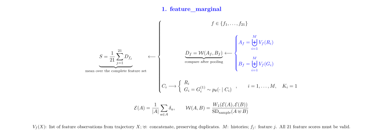
Generated continuations per history: \(K_i\in\{1,2,\ldots\}\), determined by the input files; this scoring mode does not fix a numerical \(K\). It pools feature observations from all \(K_i\) members. If each history has one generated file pair, \(K_i=1\); if each has \(K\) pairs, \(K_i=K\). Different histories may have different counts.
Question: Does each generated feature have the right overall distribution?
Step 1 — Pool before comparing
Reading the pooling symbol. \(\biguplus\) means “join all these lists and keep duplicates.” It does not add their numerical values and does not remove repeated values as a set union would.
For two histories, if \(V_f(R_1)=[1,1,2]\) and \(V_f(R_2)=[2,3]\), then
The result has five observations. Its empirical distribution assigns probability \(2/5\) to 1, \(2/5\) to 2 and \(1/5\) to 3. It is not the sum 9 or the mean 1.8.
In the next equation, \(A_f\) is the complete real feature-value list; \(B_f\) is the complete generated feature-value list. The first blue operator loops over histories. On the generated side, the outer operator loops over histories and the inner operator loops over the generated members for each history.
Difference: the context identity disappears before the distance is computed. A trajectory producing more feature observations contributes more mass to the pooled distribution. More generated members for a context also contribute more generated observations.
Step 2 — Compute one normalized distance per feature
\(D_f^{\mathrm{marginal}}\) is one scalar distance for feature \(f\) under this protocol; its superscript is a name, not an exponent.
Step 3 — Average the complete feature set
\(j\) indexes features, \(f_j\) is the \(j\)-th feature, and \(S_{\mathrm{WS21}}\) is the final equal-feature average. “WS21” labels the complete 21-feature score. For the complete 21-feature contract,
Features are equally weighted, regardless of their observation counts. A mean over fewer available features must not be silently presented as complete WS21.
What it misses. Suppose the real outcomes for two histories are 0 and 1, but the generated outcomes are 1 and 0. Both pooled distributions are \(\{0,1\}\), giving zero distance even though both historical pairings are wrong. This is the distinction between context-conditioned generation and context-agnostic scoring.
2. context_paired
Supplementary information: generated continuations and ensembles
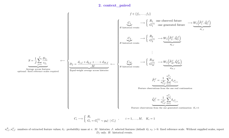
Generated continuations per history: \(K_i=1\) for every history by default in the new implementation. If multiple members already exist, select one fixed generation ID rather than choosing the best-scoring member. Multiple-member scoring requires explicit --ensemble; then \(K_i\) is the supplied member count, and the ensemble-corrected score requires \(K_i\geq2\).
Question: Does a generated future match the realized future associated with its own history?
Step 1 — Keep the context identity
The new default uses \(K_i=1\). Write \(G_i=G_i^{(1)}\) and \(\widehat Q_i^f=\widehat Q_{i1}^f\).
Difference: compute the distance inside each historical pairing before averaging across histories.
Here \(d_{i,f}\) is the unnormalized distance for one history \(i\) and one feature \(f\). The subscript \(i\) is retained so that the two distributions cannot be exchanged across histories before scoring.
Step 2 — Give each history equal weight
\(D_f^{\mathrm{paired}}\) is the arithmetic mean of those per-history distances for feature \(f\).
For scalar outcomes, \(d_{i,f}=|f(R_i)-f(G_i)|\). For event-level features, it compares within-path empirical distributions. These are different representations of a future, not interchangeable measurements.
Step 3 — Use fixed reference scales for an optional feature aggregate
\(J\) is the number of selected features; \(j\) indexes them; \(s_{f_j}^{\star}\) is a supplied positive reference scale in the units of feature \(f_j\). Dividing by it makes each term dimensionless. \(S^{\mathrm{paired}}\) is the scalar average across all selected scaled feature scores. The star labels a fixed reference, not an optimized value.
Difference: the positive scales are fixed from separate reference data and reused across models. They are not joint real/generated standard deviations recomputed for each model. Without supplied scales, the implementation reports raw feature means and leaves the cross-feature aggregate undefined. Its numerical values are not directly comparable with WS21.
The new CSV adapter supports:
| Feature | Representation |
|---|---|
| Spread | Event-level best ask minus best bid |
| Volatility | One sample standard deviation of 0.1-second log-midpoint returns per continuation |
| OFI | Distribution of 100-transition rolling order-flow-imbalance means |
| Return | One log return from the last historical midpoint to the final continuation midpoint |
These four representations are not the 21-feature contract. Insufficient observations for a requested feature cause an explicit error rather than silently becoming a zero score.
Step 4 — Optional wrong-pairing control
\(I\) is the set of histories eligible for this control; \(|I|\) counts them. \(\pi\) is a reassignment of indices within each allowed block, and \(\pi(i)\ne i\) means a history never receives its own generated continuation in the control. \(\Delta_f\) is the shuffled score minus the matched score for feature \(f\).
Reassign generated ensembles within an allowed block, such as a ticker-day, with \(\pi(i)\ne i\). On the same eligible set \(I\) on both sides,
A positive gap means correct pairing performs better on this score. Singleton blocks cannot be shuffled and their exclusion is reported. This is an offline pairing diagnostic, not an inference rerun, a permutation p-value, or a causal hidden-state intervention. Initial-book constraints and other covariates can also explain the gap.
One sample: what it does and does not establish
With one observed and one generated path, the sides have symmetric trajectory counts. But single-path discrepancy does not identify the full conditional distribution or establish calibrated uncertainty. Return and volatility reduce to absolute error. The primary output is paired_w1; pooled_w1 is identical at \(K=1\).
The implementation can bootstrap whole group_id blocks, not individual events, before recomputing equal-context means. The default ticker-day blocks need to be broadened if dependence crosses those boundaries. Fewer than two blocks yields no interval.
Optional ensembles
Multiple members require explicit opt-in. In the following equations, \(A_{i,f}\) is a scalar average distance, distinct from the pooled observation list \(A_f\) above. \(F_{i,f}\) is its ensemble-corrected score. \(k,\ell\) index two generated members, and \(k<\ell\) visits each unordered pair once; \(\ell\) here is not the lag parameter used in the next section. The implementation also reports
In the expectation expression below, \(X,X'\) are independent generated feature representations under the same history, \(y\) is the observed representation, and \(d\) is their Wasserstein distance (absolute difference for scalars). The prime marks a second independent draw, not a derivative. For independent, identically distributed ensemble members, the score estimates \(E[d(X,y)]-E[d(X,X')]/2\) without self-pair bias. It is fair CRPS for scalar outcomes and a Wasserstein energy score for empirical feature distributions. It is not a full path-distribution metric. Finite-sample scores can be negative. For \(K_i=1\) it is unavailable, not zero; the implementation reports coverage rather than silently discarding ineligible contexts.
3. feature_conditional
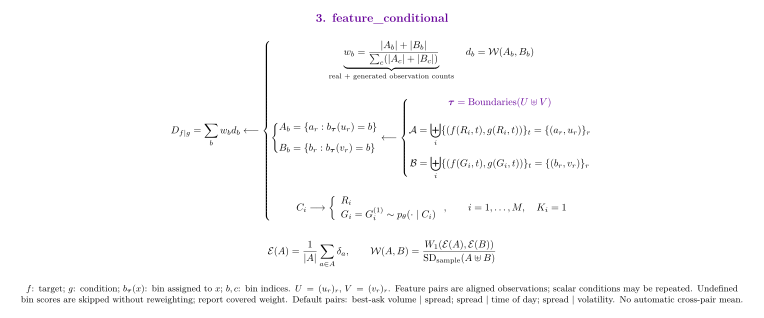
Generated continuations per history: \(K_i\in\{1,2,\ldots\}\), determined by the input files, not by the conditional scoring mode. All members contribute target-condition observations to the pooled groups. \(K_i=1\) is valid. The three configured feature pairs are three scores, not three generated continuations.
Question: Are relationships between features realistic, such as spread at a given volatility?
Example: spread given volatility
Here, spread is the target being compared, and volatility is the feature used to form groups: \(\mathrm{spread}\mid\mathrm{volatility}\).
| Comparison | Real spread observations | Generated spread observations | Question answered |
|---|---|---|---|
| Marginal | All real continuations, pooled | All generated continuations, pooled | Does spread look realistic overall? |
| Feature-conditioned: low volatility | Continuations with low measured real volatility | Continuations with low measured generated volatility | Does spread look realistic within the low-volatility group? |
| Feature-conditioned: high volatility | Continuations with high measured real volatility | Continuations with high measured generated volatility | Does spread look realistic within the high-volatility group? |
The two groups illustrate the idea; the implemented default uses the quantile boundaries described below, rather than a fixed low/high split. Both sides use the same boundaries, but each continuation is assigned using its own volatility. The within-group distances are then weighted by the real-plus-generated observation counts, as in Step 4.
To see what grouping adds, suppose low- and high-volatility groups contain equal numbers of spread observations:
| Volatility group | Real spread (ticks) | Generated spread (ticks) |
|---|---|---|
| Low | 1 | 3 |
| High | 3 | 1 |
Both pooled spread distributions contain equal proportions of 1 and 3 ticks, so their marginal Wasserstein distance is zero. Within each volatility group, however, the generated spread is wrong. Feature-conditioned scoring detects this reversed relationship even though the marginal spread distribution matches.
Step 1 — Attach a conditioning value to every target observation
\(\mathcal A_{f,g}\) and \(\mathcal B_{f,g}\) are lists of pairs, not lists of distances. Each pair contains a target value and its conditioning value. \(n_R,n_G\) count real and generated feature observations, respectively; \(r\) indexes an observation on the relevant side. Write these lists as
\(a_r,b_r\) are target values; \(u_r,v_r\) are aligned condition values. A continuation's scalar volatility can be repeated as the condition for its event-level spread observations.
Step 2 — Derive shared boundaries
\(\tau_b\) is the \(b\)-th numerical boundary, \(\boldsymbol\tau\) is the list of boundaries, and \(q\) is the number of boundaries. \(\operatorname{Quantile}_{p}(A)\) extracts the \(p\)-quantile of list \(A\); \(p=b/10\) below is a percentile level, not a bin weight. For the default continuous-condition rule,
Difference: boundaries normally come from the real and generated continuation conditions together. The percentile levels are fixed; their numerical thresholds are data-dependent. Ties mean groups need not contain exactly 10% of observations.
\(b_{\boldsymbol\tau}(x)\) is a function returning a bin ID, not a feature observation. It counts how many boundaries the numerical value \(x\) has reached or exceeded. With ordered boundaries \(\boldsymbol\tau\), the implementation's right-sided lookup is
Discrete conditions use unique observed values. Explicit thresholds override the default quantile rule. The quantile implementation also handles repeated boundaries by removing excess duplicates and applying a small offset to remaining repeats.
Step 3 — Each side groups by its own condition
The colon in \(\{a_r:\text{condition}\}\) means “keep those observations satisfying this condition.” \(A_{f,b},B_{f,b}\) contain target-feature values assigned to bin \(b\). The unadorned \(b\) is a bin ID; \(b_r\) is a generated target value. These are different quantities despite sharing a letter.
A generated observation is not assigned using its real counterpart's volatility. It uses its own condition value.
Step 4 — Compare within groups, then weight by counts
\(d_{f,g,b}\) is the distance for target \(f\), condition \(g\), and bin \(b\). \(w_b\) is that bin's fraction of all real-plus-generated observations. \(c\) in the denominator is a second bin index, used to sum over all bins without confusing it with the selected bin \(b\). \(D_{f\mid g}^{\mathrm{conditional}}\) is the resulting scalar score for one target–condition pair; the vertical bar reads “target \(f\) given condition \(g\).”
Weights count real plus generated feature observations. They are not equal-bin weights or equal-context weights. For group counts 500, 300, 200 and normalized distances 0.1, 0.2, 0.4, the result is \(0.5(0.1)+0.3(0.2)+0.2(0.4)=0.19\).
The three configured pairs
| Target | Condition | Boundary rule |
|---|---|---|
| Best-ask volume | Spread | Discrete values |
| Spread | Time of day | linspace(0, 86400, 24) |
| Spread | Volatility | Default deciles |
The time configuration has 24 boundary points, spaced about 62.61 minutes apart, not exact hourly bins. Volatility uses midpoint log returns resampled at 0.1 seconds. The scorer does not automatically evaluate every ordered pair among 21 features. An additional mean over these three pairs is a separately declared aggregate, not WS21.
Missing groups matter
The existing aggregation uses np.nansum(weights * losses). Undefined groups can be omitted without renormalizing their original weights:
“Finite” means a defined numerical value, neither NaN nor infinity. The summation subscript restricts the sum to those valid bins. \(D_{\mathrm{code}}\) is the resulting implementation output, and coverage is the fraction of original bin weight with a valid distance, between 0 and 1.
Check coverage alongside the score. Missing observations must not be interpreted as zero discrepancy. This caveat also applies to other modes using the same grouped aggregation pattern.
4. context_binned
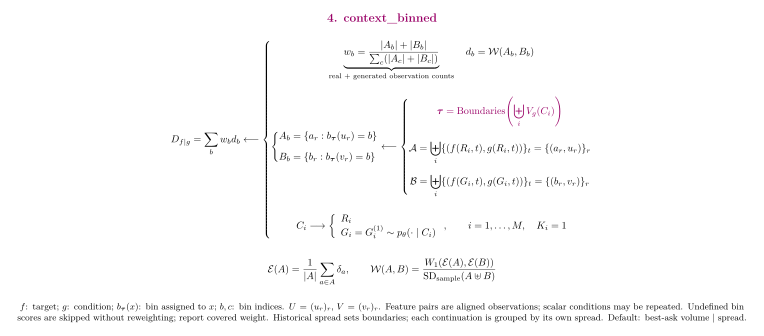
Generated continuations per history: \(K_i\in\{1,2,\ldots\}\), determined by the input files; the mode does not prescribe \(K\). All generated members are assigned to bins using their own continuation features. Historical context supplies the boundaries. The number of bins is unrelated to \(K_i\).
Question: Do continuation feature distributions match within regimes whose boundaries are derived from historical data?
Step 1 — Change where the boundaries come from
\(H_g\) is a list of historical values of the conditioning feature \(g\). \(\operatorname{Boundaries}\) means the configured rule for constructing a threshold list: in this default it takes unique historical spread values. It is not a distance or an average. \(\boldsymbol\tau\) has the same meaning as in the preceding method.
Difference: historical context determines the boundaries. The default pair is best-ask volume given spread. Because discrete=True, unique historical spread values take precedence over n_bins=10; ten groups are not guaranteed.
Step 2 — Group continuation values using those boundaries
The conditions \(u_r,v_r\) are still the continuations' own spread values. The implementation does not assign an entire future to a regime determined by its historical context.
Step 3 — Reuse within-group distances and count weights
There is one default feature pair. Crucially, this mode does not compute one distance for each historical context. The more specific name avoids confusing historical bin calibration with historical pairing.
5. time_lagged
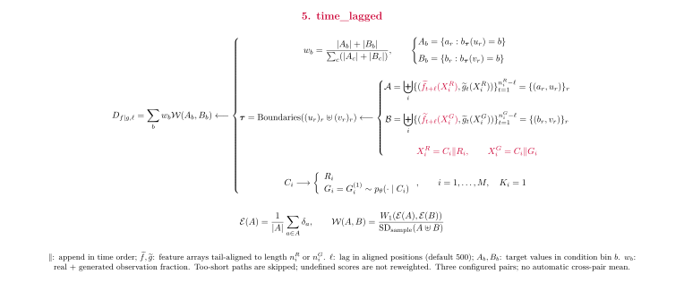
Generated continuations per history: \(K_i\in\{1,2,\ldots\}\), determined by the input files; \(K_i=1\) is supported. Each member is separately appended to the same historical context, then its lagged feature pairs enter the pooled comparison. The lag (for example, 500 aligned positions) is not the number of generated members. Too-short members may be skipped, so report the scored coverage as well as the input count.
Question: Are relationships between earlier features and later features realistic?
Step 1 — Prepend historical context
\(X_i^R\) is history \(i\) followed by its real continuation; \(X_{ik}^G\) is that history followed by generated member \(k\). Superscripts \(R,G\) label the real/generated branch. Extract target and condition arrays on the merged sequence. The implementation tail-aligns them to a common length \(n\); call the aligned arrays \(\widetilde f\) and \(\widetilde g\).
Step 2 — Offset target and condition by a lag
Here \(\ell\) is the positive lag measured in aligned array positions; \(t\) indexes an earlier position and \(t+\ell\) a later one. The tilde on \(\widetilde f,\widetilde g\) denotes the tail-aligned feature arrays. \(n_i\) and \(n_{ik}\) are the available aligned lengths for the real trajectory and generated member, respectively. \(\mathcal A_{f,g,\ell},\mathcal B_{f,g,\ell}\) collect the resulting (later target, earlier condition) pairs. This \(\ell\) is a lag, not the ensemble-member index in the preceding section.
Difference: the target occurs later than the condition. The actual slices are condition [:-lag] and target [lag:]. Slicing both arrays identically would only truncate them. For event-aligned features the lag is an event offset, not seconds; rolling or length-changing features require checking the alignment explicitly.
Step 3 — Reuse conditional binning and aggregation
\(A_{f,g,\ell,b}\) and \(B_{f,g,\ell,b}\) are the target-value lists selected into bin \(b\) by the lagged condition. \(w_b\) is calculated from these lists' real-plus-generated counts, using the same definition as before. \(D_{f\mid g,\ell}^{\mathrm{lagged}}\) is one scalar score for the target, condition and lag.
The current default pairs, each configured with lag 500, are best-ask volume given earlier spread, best-ask volume given earlier OFI, and best-bid volume given earlier OFI. They remain pooled conditional comparisons, not one score per history.
This mode is closer to a past-to-future dependency check than same-stage feature conditioning. It still does not assess every aspect of \(p(Y\mid C)\). Because scoring uses the merged sequence, targets can include historical positions when the history exceeds the lag. Too-short aligned sequences are skipped; coverage must be checked.
6. temporal_divergence
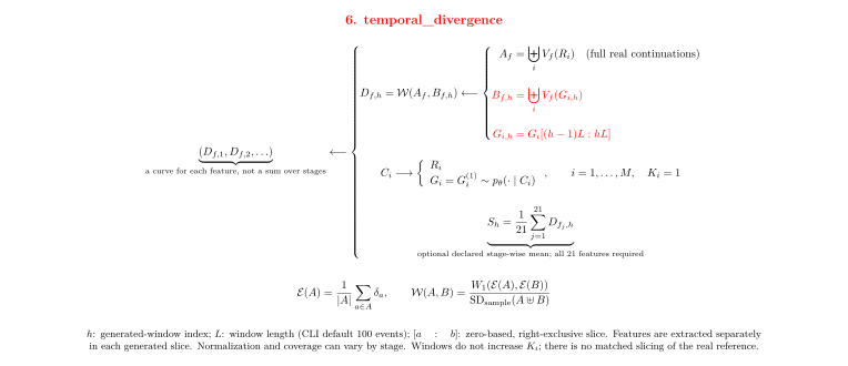
Generated continuations per history: \(K_i\in\{1,2,\ldots\}\) complete generated trajectories, determined by the input files. Each trajectory is then split into successive windows. These windows do not increase \(K_i\). A stage pools the available windows from those trajectories; later-stage coverage can differ when lengths differ. \(K_i=1\) still produces a multi-stage curve.
Question: Does feature-distribution discrepancy change as generation proceeds?
Step 1 — Slice the generated continuation
\(H\) is the number of generated events per window; \(h=1,2,\ldots\) is the window index. \(G_{i,h}^{(k)}\) is window \(h\) of generated member \(k\) for history \(i\). The slice uses zero-based positions, includes its left endpoint and excludes its right endpoint. For window length \(H\),
These are successive windows, not cumulative prefixes. The adapter's default is 100 messages per window. Available windows depend on actual sequence length and the slicing implementation.
Step 2 — Keep the full real reference
\(A_f\) is again the pooled real feature-value list. \(B_{f,h}\) pools generated feature values only from stage \(h\). \(D_{f,h}^{\mathrm{temporal}}\) is one normalized feature distance at that stage. Feature \(f\) and stage \(h\) are different indices.
Difference: only the generated side is divided by generation stage; each stage is compared with the full real feature distribution. It is not a matched comparison of real and generated windows at the same historical position.
Features are extracted separately on each generated slice. A short slice may not support a rolling feature. The joint normalization scale can also change with the stage.
Step 3 — Report a curve
The braces above collect successive values into a curve; they do not sum the stages. \(S_h\) below is a feature average at one stage. If all 21 features are valid at stage \(h\), an explicitly defined stage-wise mean is
Do not silently change the feature set when comparing stages, or collapse the whole curve to one number without specifying the temporal weights. This formula describes a stage-wise aggregate, not a claim that every historical artifact already contains it.
7. The important order of operations
Pool weights empirical distributions by their actual feature-observation counts. It becomes an equal mixture only when those counts are equal.
| Protocol | Before the distance | After the distance |
|---|---|---|
| feature_marginal | Pool all continuations | Equal mean of complete feature scores |
| context_paired | Match each observed future to its own forecast | Equal history mean; optional fixed-scale feature mean |
| feature_conditional | Bin using continuation conditions | Weight bins by real + generated counts |
| context_binned | Calibrate bins on history, group continuations | Weight bins by real + generated counts |
| time_lagged | Merge history, offset features, then bin | Weight bins by real + generated counts |
| temporal_divergence | Slice generated paths by stage | Report feature-distance curves |
No label alone proves that a model uses its hidden state effectively. A stronger causal claim needs an inference intervention that controls other inputs. These protocols measure complementary properties; their numerical scores are not interchangeable.
8. Implementation and provenance
The existing mode descriptions were checked against the sigma-0 source snapshot at 63b86a429d291acbb524043dd87193f8ecb55902. The new paired implementation and its single-sample default were checked at local commit 4c1bdef8 on feat/context-paired-20260927.
| Source file | Relevant operation |
|---|---|
| src/lobpipeline/scorer/lob_bench/run_bench.py | Default feature and mode configurations |
| src/lobpipeline/scorer/lob_bench/scoring.py | Pooling, conditional grouping, historical boundaries, lagged alignment and horizon slicing |
| src/lobpipeline/scorer/lob_bench/partitioning.py | Feature extraction tables and boundary assignment |
| src/lobpipeline/scorer/lob_bench/metrics.py | Joint sample standard deviation and Wasserstein computation |
| src/lobpipeline/lob_bench/context_paired.py | New paired scores, ensemble correction, aggregation and controls |
| src/lobpipeline/lob_bench/context_paired_io.py | Context identity, CSV pairing, feature definitions and member selection |
Historical artifacts can use different scorer revisions. Identify an artifact's own provenance before interpreting it through this guide. This page adds no measured scores and makes no change to the leaderboard's recorded mode labels or numbers.
See also the existing evaluation-mode reference, including its implementation caveats and earlier source snapshot.